

#LabHacks: Top tips for performing paired recordings
Sam A Booker, Simons Initiative for the Developing Brain, Centre for Discovery Brain Sciences, University of Edinburgh, Edinburgh, UK
A cornerstone of modern neuroscience research is understanding how neurons connect and transmit information between each other and within small working groups. Numerous technological advances have drastically increased our ability to record such connections, e.g. chemogenetics and caged neurotransmitters employed in combination with single or multiphoton stimulation. Despite the increasing use of such techniques, their implementation is often less than trivial – requiring surgical techniques, costly optical systems, a confidence that your stimulation is specific, and the ability to activate a very small number of cells to allow interpretation of the resulting synaptic responses.
For these reasons, the gold standard method to assess functional connectivity between neurons remains paired recordings. However, the mere mention of paired recordings is often sufficient to evoke cold sweats from slice electrophysiologists, but this should not be the case. This #LabHack aims to provide a number of key elements that are critical to performing this type of patch clamp recording, as well as further considerations that could extend your in vitro electrophysiology repertoire.
Before getting into the nuts-and-bolts, the aim of paired recordings is fiendishly simple: many neurons form local networks, so if we record two neurons simultaneously in that network there is an inherent probability that they will be connected [1]. The properties of these connections can then be measured to directly assess pre- and postsynaptic function. Once one has obtained such a synaptic connection, there are many different experiments that can be considered, such as: pharmacological manipulation, quantal and connectivity analysis, or synaptic plasticity. However, at the most basic level, the key pieces of information that paired recordings can provide are:
- Connection probability: the likelihood that a connection between two cells exists
- Synaptic strength: the amplitude of the synaptic response between a pair of neurons
- Short term plasticity: the ability of a presynaptic input to maintain transmitter release
These types of experiments have been employed with great success to examine the functional connectivity and plasticity of a number of neurons, their subcellular compartments, across brain regions, development, and in models of disease to name but a few [2-7]. Indeed, the process itself has been described previously [1, 8, 9]. The purpose of this #labhack is not to instruct you how to do it explicitly, but to identify the key considerations that will help you get up and running.
1. Set up your rig
It goes without saying that if you want to patch from 2 or more cells simultaneously you need to have the capability to do so. The overall rig layout is much the same as for conventional single cell recording, you need a good compound microscope with either IR-DIC or Dodt optics (Scientifica SliceScope), low (4x) and high (40x) magnification objective lenses, and a high-resolution digital camera to view the slice under (SciCam Pro). Then you need manipulators, which should be ideally low profile, allow rapid electrode changes, and automatic repositioning of pipettes (MicroStar manipulators are excellent for this). You want to position the manipulators in such a way so that you can easily access each to replace pipettes. Then you need as many amplifiers as you want cells, the Multiclamp 700B is ideal for this as it has two built in patch channels, allowing easy and rapid control of two cells. Remember, you need to have a reference electrode for each headstage amplifier – consider using a common ground electrode to save space. Next, you need pressure control for each electrode holder you plan to use. For up to four electrodes, this can be managed with individual set-ups, but if you wish to patch upwards of four cells, a more complex arrangement may be necessary [10]. The final consideration is physiological saline flow rate and temperature. As you will have multiple electrodes and cells recording simultaneously, balancing maintenance of physiology and slice stability are crucial. 6 - 8 ml/minute is a good middle ground that meets both demands [11].
2. Learn to patch reliably
This might sound obvious, but there is no point starting out planning to do multiple patch-clamp recordings from day one having never done one before. You need to be completely comfortable with your rig, the software, and the overall whole-cell patch-clamp process. I normally recommend >90% successful recording from cells to target as a goal. This is important, as the last thing you want is to attempt to record multiple post-synaptic cells without success, while a healthy pre-synaptic cell is recording. Furthermore, once a stable pre-synaptic neuron is recorded, you may want to record multiple post-synaptic cells, which requires a high reliability of achieving a whole-cell recording.
Read Scientifica's 14 sharp tips for patch clamping here
3. Identify your target circuit/cell type
Beyond technical set-up and recording ability, a major consideration for successful paired recordings is choosing your brain region or preparation to record from. As the purpose of paired recordings is to assess native synaptic connections, the majority of studies are performed in acute brain slices. However, in a brain slice the likelihood that such connections have been spared during the slicing depends on whether the connections are local or long range, and if the presynaptic axons are likely to be maintained in the slice. If they are not, you could conceivably record hundreds to thousands of pairs of neurons with minimal chance of a successful pairing. This is not to say that a connection does not exist, just that the technical limitations preclude recording it. When designing a paired recording experiment, it is critical to research whether anything is known about the dendritic and axonal arborisation patterns of those neurons already – or if any hint can be found in anatomical studies. However, connection probability can vary a lot between cell types, ranging from below 1% to over 50%. This is an important consideration for your first paired recordings – it is demoralising to hunt for synaptic coupled pairs of neurons if only one connection might exist for every hundred pairs of cells recorded. It is a much better idea to get a handle of the technique on neurons that are highly connected (i.e. neocortical L2/3 pyramidal cells).
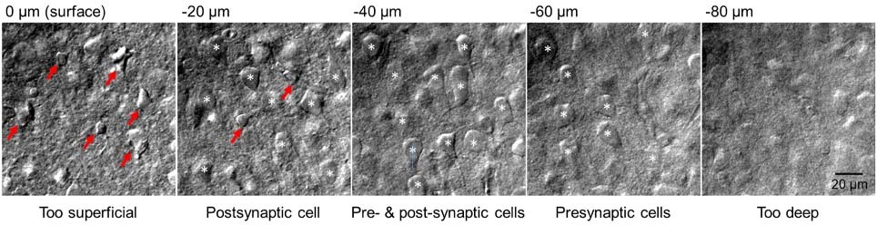
4. Slice quality, slice quality, slice quality
There is little to no point in attempting paired recordings until your slices are optimised for your brain region of choice. What you are aiming for is a slice that is flat with a lightly cratered surface and with very few, highly contrasted, collapsed cells on the surface. Immediately below, you want to see a multitude of plump and round cell bodies (Figure 1) which seal almost instantaneously upon pipette pressure release. How you achieve such quality depends on tissue type, brain region, developmental stage, and cells targeted. Recordings from younger animals tend to have more consistent high-quality cells, but might not address your research question. Likewise, a protocol that works brilliantly for neocortex may not be appropriate for midbrain structures. A number of studies which improve slice quality are available for a variety of ages and are worth perusing [9, 12, 13].
5. Solutions – getting the right balance
As with all electrophysiology experiments, regardless of type, a critical consideration is that solutions such as artificial cerebrospinal fluid (ACSF) and the solution used to slice the brain in, are sterile and balanced to the osmotic strength of neurons. This improves slice quality and the ability of the recorded neurons to be maintained in whole-cell configuration for an extended period of time. For identifying synaptic currents, you need extracellular calcium ions (~2 mM, but this depends on experiment) and you need glucose and oxygen to maintain slice viability. Pre-warming your buffer before perfusing around your rig facilitates oxygen/carbon dioxide saturation and makes for a more stable bath temperature. An ideal osmolarity of ACSF should be 300-320 mOsm, with a pH of 7.3-7.4 following bubbling with carbogen. Maintaining the bath temperature at 30-32 °C through the use of an in-line heater allows for large amplitude, fast synaptic currents, which have a physiological reliability.
6. Identifying your cells of interest
As mentioned in point 3, different cell types possess quite diverse connection probabilities and often even more divergent pre- and postsynaptic functional properties. To reliably sample as many cells of interest, you may want to consider using a rodent model that expresses a fluorescent reporter under a promotor specific to the cells you are interested in. For example, if you are interested in the connectivity of inhibitory neurons, a fluorescent tag (e.g. red td-Tomato) can be expressed under an interneuron specific promotor (e.g. PV, see Figure 2A), thus allowing you to reliably identify inhibitory interneurons as fluorescently labelled and excitatory neurons as non-labelled cells. A multitude of different reporter lines now exist, which can be chosen specifically for your target cells and general experimental design.
7. Inhibition or excitation – solutions are the solution
Given their high connectivity and role in local processing, inhibitory GABAergic interneurons are often recorded during paired recording experiments (Figure 2A), as this allows an easy mechanism to understand local circuit processing [7]. However, recording synaptic GABAA receptor mediated currents originating from interneurons requires further consideration as the native reversal potential for chloride ions in mature neurons is often close to the resting membrane potential (-60 to -70 mV), thus measuring synaptic responses from such a potential may be difficult. There are two alternative routes to address this problem. First, you can use an internal solution that contains a high concentration of chloride ions (<20 mM), thus pushing the driving force of the current in the depolarising direction. Alternatively, you can record your post-synaptic cells at a more depolarised membrane potential (e.g. -50 mV, Figure 2C) to evoke an inward and hyperpolarising chloride current. Either approach works well to give high signal-to-noise recordings of inhibitory postsynaptic currents.

8. Avoiding false negatives
Once you have performed a successful paired recording experiment, you want to extract as much information from those cells as possible, which includes morphological analysis. This serves two important purposes. First, you can confirm the identity of the cells recorded. Second, you should identify if the recorded neurons possessed an intact axon. The latter is a critical step to confirm the true connection probability, as if the axon was cut during slicing, this would lead to a false-negative connection. Post hoc visualisation of recorded neurons can be achieved with the inclusion of an intracellular label – such as a non-endogenous marker (e.g. neurobiotin or biocytin) or a fluorescent molecule (e.g. AlexaFluor 488 or 568). These markers can then be visualised offline with methods such as streptavidin binding combined with fluorescent microscopy [9, 14].
9. Don’t miss out on small responses
Neurons often have complex dendritic structures, with synapses formed at high electrotonic distance from the soma. Therefore, single recording traces may possess low signal-to-noise and high variability, thus detection of a synaptic connection might be prone to error, which is exacerbated by potential low release probability of synaptic connections. To ensure faithful identification of synaptic connections, it is often best to record a number of sweeps of pre-synaptic action potentials, at moderately high frequency (e.g. 10 trains of 5 action potentials delivered at 20 Hz). A trace average can be then quickly made while the cells are still both “on patch” to determine whether a connection is present (Figure 2C). This ensures that, even for small amplitude, low probability synaptic connections, a fair assessment of these connections can be made.
10. The first cell is the deepest
No matter how many cells you wish to record from simultaneously, you will likely have a target connection in mind – e.g. basket to pyramidal cell, pyramidal to pyramidal cell. As such, targeting the right presynaptic neuron is vital (see above), however for the reasons of cell viability and axon integrity it is also important to choose an optimal presynaptic neuron. This is best achieved by choosing your presynaptic neuron as deep within the tissue as you are able to achieve a stable whole cell recording. Due to the vagaries of the acute slice preparation, the deeper you can record this first presynaptic neuron the more likely the neurons axon is preserved in an in vivo condition. You can then record more superficial postsynaptic cells, which introduced less mechanical disturbance to the initial cell, but increase the innate probability of connection. In this fashion, one can with relative ease record from 5-10 postsynaptic neurons for a given presynaptic cell – allowing quick and accurate identification of the target connection.
What is outlined above should provide the detail and suggestions needed to successfully perform paired synaptic recordings from neurons in acute brain slice preparations. The relative success of such recordings is high in brain areas and cell types that have been well described. However, if the connection probability is low or you wish to sample connections from the sider network there are a new selection of emerging techniques available to up the odds of success. One “joy” of performing paired recordings, as described above, is that you never know if a connection exists before breaking-through into whole-cell configuration. If such mystery is not your cup of tea, this can be overcome either by combining a paired recording approach with single-cell optogenetic or glutamate uncaging to stimulate many potential presynaptic neurons [15] before deciding on a pair to record. However, these approaches are costly and quite time consuming. A further option is to tip the odds in your favour by simply recording many more cells simultaneously (4 - 12 neurons), which in part overcomes low-connection probability and allows more precise characterisation of the local circuit [10]. However, this requires significant rig upgrades to include multiple amplifiers and micromanipulators, as well as the time required for the experimenter to become technically competent with such a system.
Other useful electrophysiology guides
- SciMethods: Simultaneously recording from four neurons using PatchStar and MicroStar manipulators
- #LabHacks: 14 sharp tips for patch clamping
- Using cell-attached patch clamp to monitor neuronal activity
- #LabHacks: Tips for performing adult animal brain slicing for patch clampers
- #LabHacks: Tips for successful patching of immature embryonic and young postnatal neurons
- Tips for reducing pipette drift in electrophysiology experiments
- Patch clamp techniques for investigating neuronal electrophysiology.
References
- Miles, R. and J.-C. Poncer, Paired recordings from neurones. Current opinion in neurobiology, 1996. 6(3): p. 387-394.
- Ali, A.B., et al., CA1 pyramidal to basket and bistratified cell EPSPs: dual intracellular recordings in rat hippocampal slices. The Journal of Physiology, 1998. 507(1): p. 201-217.
- Bartos, M., et al., Rapid signaling at inhibitory synapses in a dentate gyrus interneuron network. Journal of Neuroscience, 2001. 21(8): p. 2687-2698.
- Grosser, S., et al., Parvalbumin interneurons are differentially connected to principal cells in inhibitory feedback microcircuits along the dorsoventral axis of the medial entorhinal cortex. Eneuro, 2021. 8(1).
- Hefft, S., et al., Presynaptic short‐term depression is maintained during regulation of transmitter release at a GABAergic synapse in rat hippocampus. The Journal of physiology, 2002. 539(1): p. 201-208.
- Peng, Y., et al., Layer-specific organization of local excitatory and inhibitory synaptic connectivity in the rat presubiculum. Cerebral Cortex, 2017. 27(4): p. 2435-2452.
- Savanthrapadian, S., et al., Synaptic properties of SOM-and CCK-expressing cells in dentate gyrus interneuron networks. Journal of Neuroscience, 2014. 34(24): p. 8197-8209.
- Wilms, C.A., Therese; Sjöström, Per Jesper Simultaneously recording from four neurons using PatchStar and MicroStar manipulators. SciMethods.
- Booker, S.A., J. Song, and I. Vida, Whole-cell patch-clamp recordings from morphologically-and neurochemically-identified hippocampal interneurons. Journal of visualized experiments: JoVE, 2014(91).
- Peng, Y., et al., High-throughput microcircuit analysis of individual human brains through next-generation multineuron patch-clamp. Elife, 2019. 8: p. e48178.
- Hájos, N. and I. Mody, Establishing a physiological environment for visualized in vitro brain slice recordings by increasing oxygen supply and modifying aCSF content. Journal of neuroscience methods, 2009. 183(2): p. 107-113.
- Bischofberger, J., et al., Patch-clamp recording from mossy fiber terminals in hippocampal slices. Nature protocols, 2006. 1(4): p. 2075-2081.
- Ting, J.T., et al., Acute brain slice methods for adult and aging animals: application of targeted patch clamp analysis and optogenetics, in Patch-clamp methods and protocols. 2014, Springer. p. 221-242.
- Oliveira, L.S., A. Sumera, and S.A. Booker, Repeated whole-cell patch-clamp recording from CA1 pyramidal cells in rodent hippocampal slices followed by axon initial segment labeling. STAR protocols, 2021. 2(1): p. 100336.
- Beed, P., et al., Analysis of excitatory microcircuitry in the medial entorhinal cortex reveals cell-type-specific differences. Neuron, 2010. 68(6): p. 1059-1066.
)